Simulation
Neural Network Training
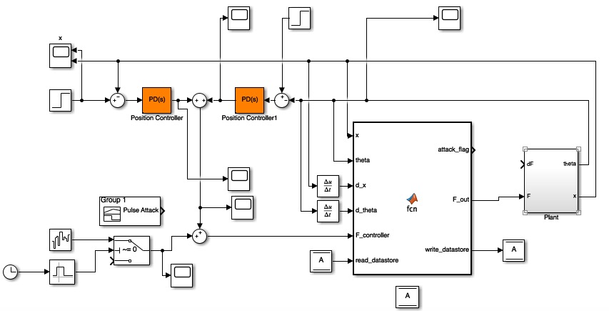
We set up the simulation of the training process using Matlab and Simulink. The Simulink model used for this stage of the experiment is given below:
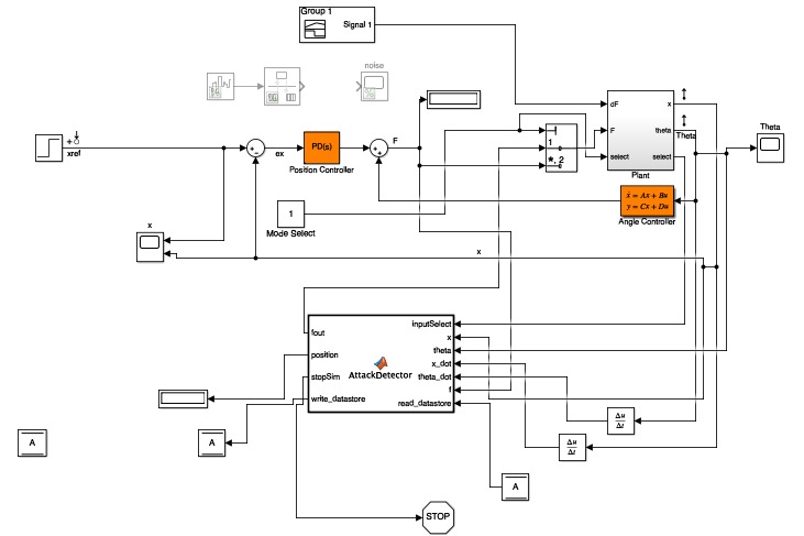
The primary Simulink block labeled AttackDetector (actually a misnomer) consists of the logic that was run per episode of the training. The primary point to note here is the feedback loop between the training block and the plant (the actual pendulum), and its relation to the main program which was running the reinforcement learning algorithm. At the start of an episode, the neural net was constructed based on the parameters it was trained with by the reinforcement learning algorithm during the previous step. Once this network was available, the plant ran through roughly either 900 steps or until failure (pendulum falls beyond 90 degrees from apogee) to record data points. During each step the plant iterated through all of the possible 81 discretized actions (which we had to artificially declare since there was no way to declare a continuous set of actions) to determine the best possible action for the plant's current state based on the q-value output by the neural network for each state-action value pair. Addtiionally, the training was biased largely in favor of exploration during the early training steps which then eventually curtailed in favor of exploitation in the later steps. This process was repeated for all steps in the current episode and sent back to the main program, which in turn used the history of the run to compute the reward for each state-action pair to serve as the basis for running SARSA reinforcment learning. The history was updated and checkpoints saved as needed before the cycle repeated itself for however many episodes we wanted to train the nerual network for. We note here that the SARSA update used the reward computations of the current run as well as the reward from the action taken in the next run in a backwards-looking approach as opposed to Q-Learning which simply selects the optimal reward-yielding action in the next state. Based on both empirical testing and some theoretical basis, we believed that SARSA yielded more realistic results and would necessarily result in the agent moving further away from actions that would result in actions that would result in very negative scores, even if the optimal action was very close to a "dangerous" state. An illustration of the difference can be found here[1].
NOTE: All code used for this portion of the project can be found here.
Attack Detection
Following the completion of the training phase, we switched the controller of the pendulum setup. During training, the neural network was allowed to completely control the setup in order to populate and update the Q values based on a variety of desirable and undesirable states; however, its main purpose is to serve as a guard in monitoring the behavior of an actual system controler (in our case, this was a PID controller). A PID controller (or rather a linear controller and an angular controller combined) was thus given control over the system with the neural network layered on top of the control scheme. The Simulink model used for this stage of the experiment is given below:
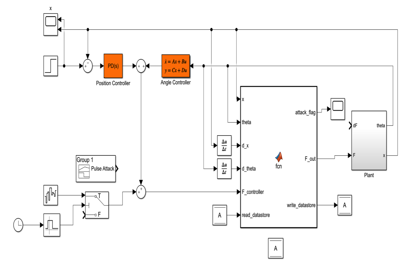
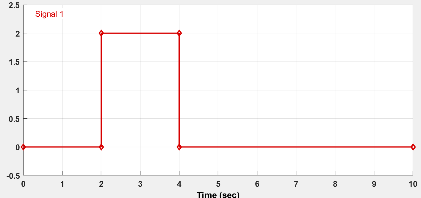
At several seconds into the simulation, an artificial attack was introduced into the system which took the form of an impulse. This resulted in a signficant drop in the health scores and was detected as an anomaly / attack by the network. The following image represents the waveform of the attack:
The video below visually simulates the effect of this attack on the system:
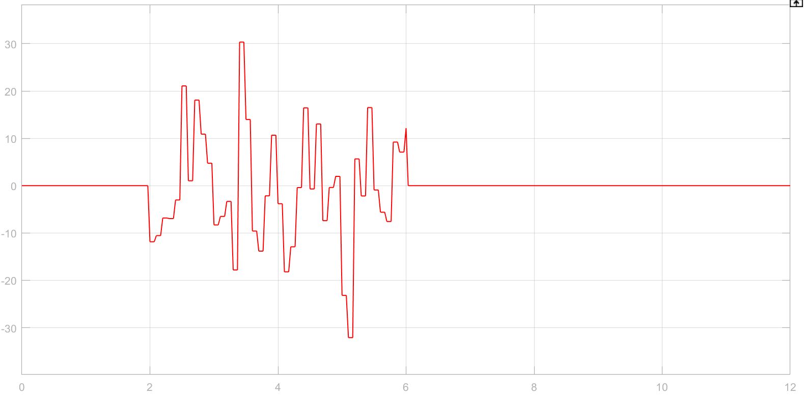
To explore more than one possible attack, a white noise attack was introduced as well. This resulted in a large amount of volatility in the health scores and was thus also detected as an anomaly / attack by the network. The following image represents the waveform of the attack:
Additionally, the profiles of the simulated attacks and the resulting health score profiles (which is equivalent to a score out of 100 representing the ratio of posible state-action pairs compared to the total number of possible pairs that the controller's decision performs better than):
The video below visually simulates the effect of this attack on the system:
The optimally selected attack detection algorithm and its results will be discussed in the Results section of the site.
NOTE: All code used for this portion of the project can be found here.
Attack Correction
The final step of the simulation phase was the attack corrector, which involved the handing off of system control between a PID controller and a trained neural network. The Simulink model used for this stage of the experiment is given below:
Not surpringly, this schematic looks nearly identical to that used for the attack detection (besides the core logic in the large block being different); however, there is noteworthy difference in the replacement of the original angle controller by a second PID. Essentially, we attempted to use a linear controller for a nonlinear system, which resulted from the handoff of the NN back to the PID and vice versa. This caused caused the angle state space controller to degenerate and the health score rapidly dropped to 0 as a result. Replacing the angle state space controller with the second PID solved this problem.
The attack correction algorithm was run with the aforementioned white noise attack. The results of the simulation, as well as an illustration of the health score degeneration problem, will be discussed in the Results section of the site.
NOTE: All code used for this portion of the project can be found here.
Physical Testbed
NOTE: The physical testbed code is fairly segmented. Follow the instructions on the main README of the github repository to build the folder to be exported to the target and to make the appropriate test to be run. The host computer running Matlab is only needed for the training portion of the experiment - all code for the host can be found here. Almost all of the testbed code is written in C to optimize performance, with an occassional shell script or two to perform setup or provide wrappers.
Setup
The physical testbed was constructed using a combination of mechanical parts and electronics. The primary chassi was based on the Channel Slider Kit B from Actobotics; however, many components needed to be added or removed to construct the final setup. The front view of the setup is pictured below:
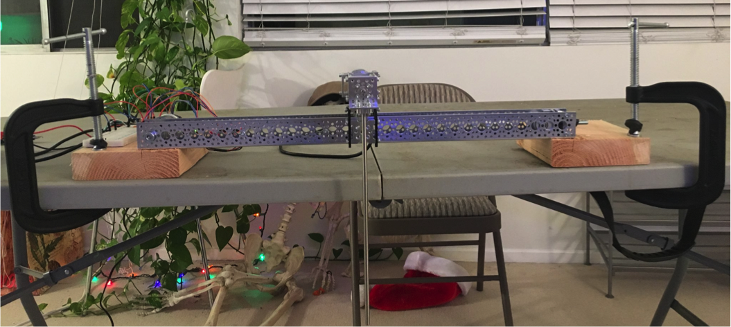
Unlike most inverted pendulum setups, the length of our main channel was only about 2 feet, with several inches removed to clamp the setup to the two wooden boards at the ends. This resulted in our structure needing to impose significantly tighter constraints on the value of x, which we will discuss further in the results. The slider itself was a rubber belt wrapped at both ends by simple pulleys. Teeth-like protrusions from the belt fit into the grooves of the pulleys to provide traction during sliding. The wooden boards at the sides along with the industrial clamps were intended to prevent the entire slider from being overwhelmed by the force exerted by the DC motor and to serve as a panel to which the majority of our electornics could be attached. The pendulum itself is about 1 foot in length, which also made it a fair bit shorter than a large number of the pendulums used in other projects.
The below photo provides a zoomed in view of the mounted component on which the pendulum itself moves linearly:
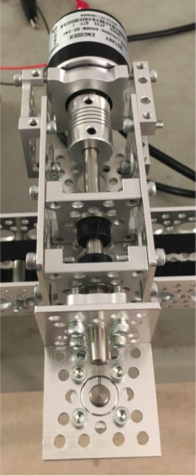
The rotary encoder (used to determine angular position) was connected to the swinging mount via a shaft coupler, with several components in between to serve as extra support to prevent shifting during motion.
Pictured below are all of the electronics used as controllers, sensors, and actuators in the system. All components are labeled for clarity:
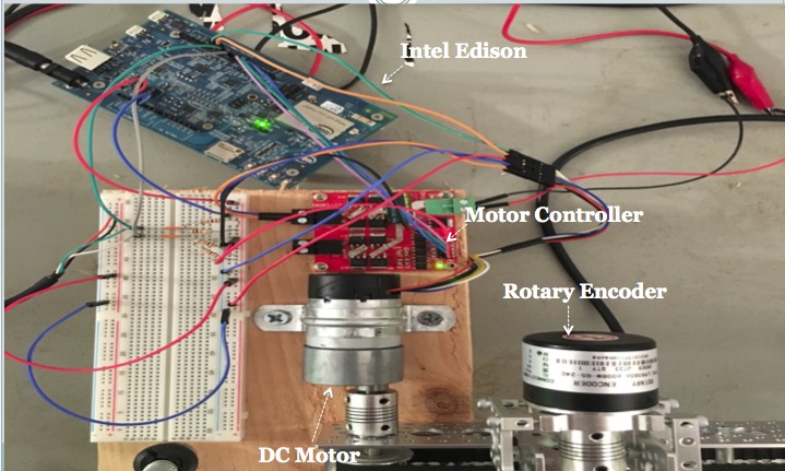
The DC motor served as the primary driver of the slider, with the embedded hall sensor serving to approximate position since the DC motor itself has no concept of distance traveled. The motor, rotary encoder, and motor controller are all connected to the Intel Edison, which serves as the priary controller. The following diagram represents a schematic view of this system:
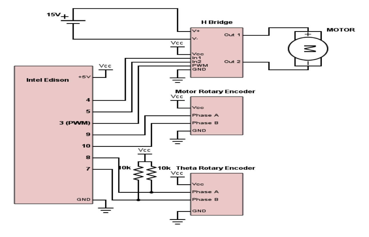
The majority of the electronics operated at 5V and could thus be driven directly by the Edison. However, the DC motor could operate at a significantly higher level of 16V. In order to get the motor to move and respond as fast as possible, we wanted to supply it with the maximum amount of voltage it could tolerate. For this reason, we decided to use an external variable voltage source to drive this single component in the system while keeping the other components fixed to 5V. We also neede a couple of pull up resistors to cleanly separate logical low and high for the pulses interrupts transmitted by the rotary encoder due to our extreme dependence on accurate angle measurements.
Finally, our target device software architecture can be represented by the following diagram:
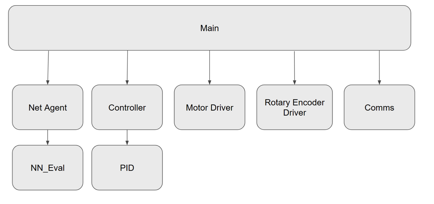
Net_Agent and NN_Eval contain the portions that interact with the neural network as well as computation of the optimal action among the set of all possible actions for a given state. The PID controller contains the core logic for the control flow during standard operation in the attack detection and correction phases. The communication block serves as the wrapper to communicate with the host during training, while the remaining two components are the drivers used to interact with the physical actuators and sensors on the system. The Kalman Filter is implicitly embedded into the rotary encoder driver to help smooth out the interrupt pulses for accurate angle mearsurement, though it hardly can be considered a good one.
Neural Network Training
Since the reinforcement learning portion of our NN training was deeply tied to our Matlab simulation implmentation, we wanted to leverage our existing work to train the physical system. Unfortunately, we could not use the trained NN output from the simulation since the system dynamics were completely different from the simulation. Due to the need to reuse our existing work, we needed to construct a solution in which the Edison essentially ran a C-code version of our Simulink logic block in addition to a communication system that could automatically transmit the NN to be used in the next episode when the results of the previous episode had been incorporated into the RL history. Our solution to these problems are illustrated in the following schematic:
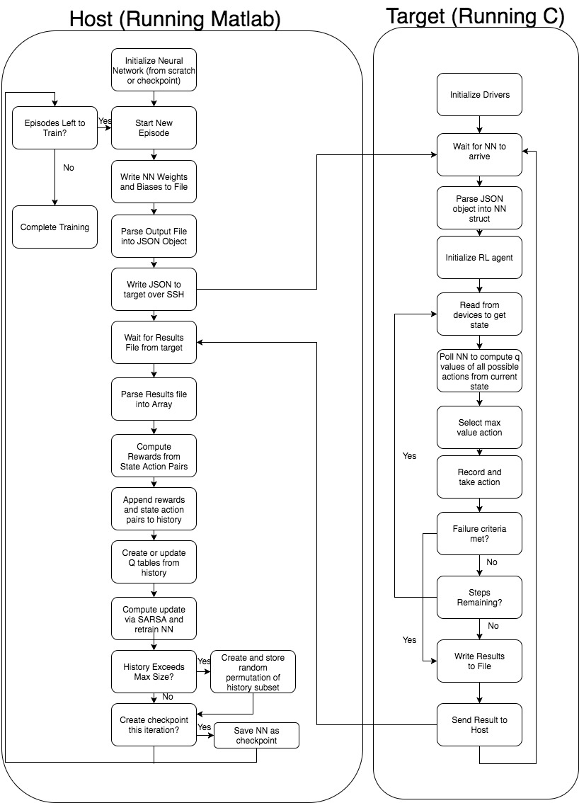
In order to prevent the testbed from needing to poll a NN that lives exclusively on the host, we decided to construct a compartmentalized representtion of the NN in a compressed JSON object and send it to the host at the start of each episode. The target device would then parse the object and reconstruct its own representation of the NN internally, while providing an easy-to-use API for other programs to use when the state-action value pair score needed to be computed. The Matlab portion functions almost identially to the simulation, except for the write operation of the NN sent over the LAN to the target device at the start of each episode rather than to a Simulink block. The target essentially echoes the function of the Simulink training block and writes the results of each run back to Matlab upon completion. Both the target and the host have listeners attached to the specific files which are to be overridden per episode, thereby providing an event-driven as opposed to time-driven loop. As stated previously, the primary goal of this phase is to train a NN that will be used as the source of truth and security guard for the remaining phases tuned to the specific system dynamics of the physical testbed.
One important point to note here is that we did not plan for needing to solve the "swing up" problem in our initial project scope. While starting the pendulum in the upright position at the start of each training run in the simulation was simply a matter of tweaking a parameter, gravity cannot be temporarily ignored in the physical world. In order to stay consistent with our simulation, we thus needed to manually readjust the pendulum to the upright position after each success or failure - a task that proved to be quite painful.
PID Tuning
While not really addressed in the simulation beyond a simple block in a simulink diagram, a PID controller would need to be actually implemented on the physical testbed. It was therefore necessary to tune the parameters of the controller system with the necessary values required to keep the pendulum stable in an upright position. This process, as we found out upon further research, was ultimately a game of guess and check. Specifics of this process will be discussed in the Results section.
Attack Detection
The following schematic illustrates the attack detection process with a trained NN:
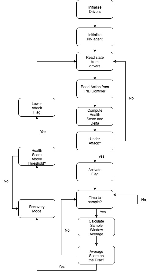
The attack detection and correction phases run exclusively on the target device, and thus translating from simulation to C code was necessary. Functionally, this operates in the same manner as the Simulink block, with the chief differences being that the polled Neural Network is a translation of the output from Matlab on the host and the values needing to be read directly from the device drivers rather than a simulation array of values.
An important point to note here is that while the code has been written for this portion, testing requires a completely trained NN and a bulletproof PID implementation. As we will discuss in the Results, these objectives were not achieved fully by the conclusion of this project. This component therefore remains largely untested beyond basic compilation and running.
Attack Correction
Finally, we have our physical testbed implementation of attack correction:
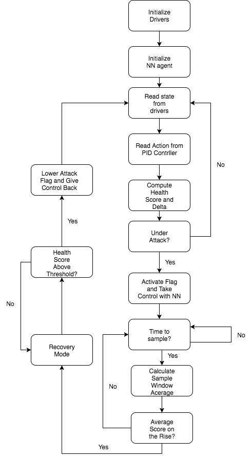
Similar to the simulation, the attack correction flowchart is largely identical to the attack detection flowchart with the chief difference being that a high signaled attack flag actually invokes action on the part of the NN rather than just serving as an alert. Due to the code requirements being almost identical, much of this component would mainly just serve as an add on to the attack detection code. Also as with attack detection, the functionality would maintain the same behavior as the Simulink block.
Unfortunately, this portion has not yet been implemented as doing so would require sound operation of the remaining components. Since the attack detection module has not yet been tested, it would take some time before this is ready to be implemented and tested. However, doing so would require only marginally more work, though certainly a non-trivial amount of testing.
References
[1] STUDYWOLF, “REINFORCEMENT LEARNING PART 2: SARSA VS Q-LEARNING” [Online]. Available: https://studywolf.wordpress.com/2013/07/01/reinforcement-learning-sarsa-vs-q-learning/. [Accessed: 15-Dec-2017].